information in this document is preliminary
v.0.31 May 13 2009 Jaakko Koivuniemi
The NMR tools were originally a collection of C++ scripts written in the CERN Root Object-Oriented Data Analysis Framework to analyze the thermal equilibrium signals, plot polarization from SPS periods and to extract different parameters from the measured signals, e.g. the center frequency of the NMR-line. These scripts were used to determine the target polarization and to check the quality of the recorded NMR data. Modifying and/or rewriting these scripts is however laborious and the NMR tools try to give the necessary tools to do the most important analysis relatively easily. These scripts and tools were used to analyze the single NMR line data of 6LiD and proton in NH3.
The total number of lines in the Ntools is now 17890.
Rather that defining own classes, methods or libraries only standard
Root libraries are used.
For faster execution the programs are compiled and linked to the Root
libraries. The compiled code goes through more strict checks than
the interpreted code making it more robust. This allows also piping
the commands on the unix shell and executing them as batch jobs.
The compiling and installation is explained in Ntools/README file.
You should also execute the test programs first without GUI and later
with GUI before starting to use the programs.
To have access to the NMR data you need an account on na58pc057. You can ask it from the administrator of that computer. Alternatively you can use the NMR signal files recorded on CDs. The amount of recorded NMR data is now
2.5G    2001
4.2G    2002
5.3G    2003
5.9G    2004
1.8G    2006
3.1G    2007
giving the total amount of 22.8 GB.
After logging into na58pc057 you can open the manual page
'man nmrtools' for general introduction to these tools.
If the result is not what you expect increase the verbose level with
switch -v to see where the problem is coming from. It
could be also that you did not use the right combination of the
input parameters for the program. These are explained in the manual
page for each program and you can get quick help by typing
the command without any parameters, e.g.
plotsig
usage: plotsig -SIGFILE [-bBGRFILE] [-sWIDTH | -wWIDTH] [-NN] [-lN] [-fFITTYPE] [-LN] [-I] [-g] [-d] [-e] [-c] [-pPHASE] [-rN] [-o] [-B] [-O] [-T] [-MN] [-vLEVEL] [-V]
        -SIGFILE signal filename
        -bBGRNAME background filename
        -sWIDTH subtract linear baseline, exclude WIDTH kHz from center
        -wWIDTH subtract parabola baseline, exclude WIDTH kHz from center
        -l number of baselines to try, default is one
        -N coil number, default 1
        -f fit G gaussian, M memory, 3 gaussians, N NH3 function
        -L fit limits: default D/6Li, 1=p, 7=7Li, -1=no limits, or initial polarization for NH3 fit 0.0 - 1.0
        -I do not fit, show initial fit function
        -g no graphics output
        -d calculate and plot dispersion signal
        -p phase correction in rads
        -e baseline noise
        -c extract solenoid current
        -r remove N points from beginning
        -o result data to standard output
        -B don't subtract fitted baseline, show fit
        -O read old SMC '.dat' format
        -T ascii text plot on terminal
        -M search for peaks with threshold 0.0 - 1.0
        -v verbose level 0 - 3
        -V version
A simple secured telnet connection is necessary to get numbers from the NMR signal and background files. After saving the result data in unix file it can be plotted later in some other environment using for example Mathematica or Matlab. For the plots with the NMR tools you need a X-windows connection from your computer. This can be done with Exceed in Windows, but the best performance is achieved with Unix, Linux or Mac OS X computers.
The Root GUI allows saving of the plot in almost any format and can also be used to add graphics or annotations to the plot.
It is also possible to run the Root in Windows, Solaris and Mac OS X and compile the NMR tools in these platforms, but this has not been tested and some programs use pipes and time functions from the Unix shell.
For the description of the CW NMR data acquisition system you can check the
reference [1] below. During physics data taking the NMR signals are recorded
every 1 - 30 minutes to the computer. The data acquisition is done with a
LabVIEW program.
The signal file has a '.sig' suffix. It is a simple
ascii file with frequency in the beginning of each line followed by the
signal amplitudes for the 10 different coils. In the data of 2001
there are actually 16 channels of which only the first 10 are meaningful.
Usually there are 1000 different frequency points.
At the end of the file there are lines that start with
'#'.
These data fields tell about the status of the Q-meters, target solenoid
current and dilution cryostat temperatures at the time of
the NMR data taking. This data may however in some cases be corrupted
if the socket connection to the magnet or dilution cryostat
computer was broken at that time. The background files with suffix
'.bgr' were recorded with the magnetic field set to a value
outside of the nuclear magnetic resonance region. Usually the background
file is subtracted from the signal file before any further analysis
of the signal is done.
A typical NMR file from run 2007.
106118000.000000        -206.962494     -206.962494     -203.462494     -200.362503     -202.737503     -204.274994     -200.850006     -205.937500     -222.149994     -207.024994
106118600.000000        -205.949997     -207.287506     -201.975006     -200.574997     -201.449997     -201.962494     -200.137497     -204.725006     -222.500000     -207.149994
...
106717400.000000        -185.449997     -194.449997     -199.562500     -176.074997     -192.412506     -200.524994     -190.787506     -196.162506     -212.762497     -186.824997
#frequency 106418000
#scan width 600000
#channels 1000
#sweeps 5
#seep up 1
#seep down 1
#trig/ch 8
#gain 0
#dc-offset trigger 1
#magnet current (A) 651.206349
#dc_monitor_1 2.790527
#dc_monitor_2 2.609863
#dc_monitor_3 2.705078
#dc_monitor_4 3.115234
#dc_monitor_5 2.644043
#dc_monitor_6 2.412109
#dc_monitor_7 2.480469
#dc_monitor_8 2.559814
#dc_monitor_9 2.460937
#dc_monitor_10 3.099365
#TTH4 (Ohm) 29810.000000
#TTH4 (K) 0.057987
#TTH6 (Ohm) 41400.000000
#TTH6 (K) -99.000000
#speer up (Ohm) 29400.000000
#speer up (mK) 69.742214
#speer down (Ohm) 18977.000000
#speer down (mK) 81.126486
#baratron (V*10) 0.040000
#9/4/2007 4:43:16 PM
#
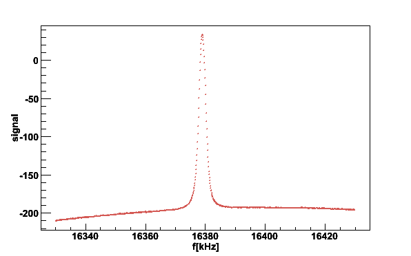
As an example we want to plot the NMR signal of coil #2 from a file of 2002 run recorded on June 19 at 17:23:23:
cd /home/NMRdata/2002/cdrom21
plotsig -020619_172323.sig -N2
Here -020619_172323.sig is the signal file name
and -N2
tells to plot the coil #2. This results to the plot
Fig 1. NMR signal from coil #2.
Next we subtract the baseline taken June 19 at 16:09:30 from the signal file
plotsig -020619_172323.sig -b020619_160930.bgr -N2

Fig 2. NMR signal after baseline subtraction.
To remove the linear residual baseline we exclude 40 kHz from the center
for the fitting with the switch -s40
plotsig -020619_172323.sig -b020619_160930.bgr -N2 -s40
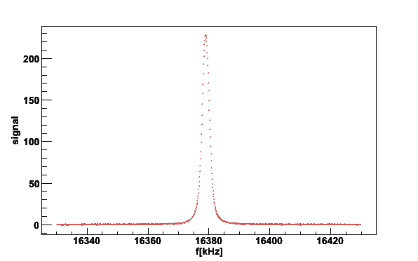
Fig 3. NMR signal after removal of residual linear baseline.
Finally we fit the signal to a memory function and extract the fitting parameters using the verbose level 2
plotsig -020619_172323.sig -b020619_160930.bgr -N2 -s40 -fM -v2
        f0      A       M2      M4      a       chi
Raw     16379   7706.28
Gaus    16379   6999.71 1.56786 -               223.016 5995.3
Initial parameters for Memory function
f0=16379 Hz a=-1.3381e+06 M2=2.5 kHz^2 M4=31 kHz^4 Gchisq=5995.3
Mem     16379   7369.28 2.33056 24.8709 -1.47386e+06    1452.52
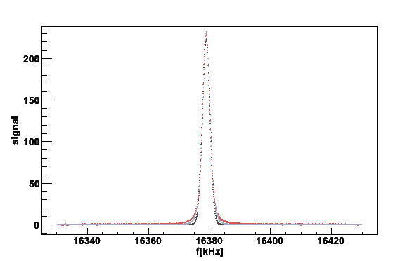
Fig 4. Gaussian and memory functions fitted to the lineshape. The black line is a Gaussian prefit and the gray the fit to a memory function.
The parameters on the screen are: f0 the center frequency of
the fitting or the first moment of
the raw NMR signal. M2 and M4 are the second
and fourth moments from the fitting, respectively. They are in units
kHz^2 and kHz^4. The A is the
integrated surface area of the raw signal or the fitted function and
the a is the amplitude in for the fitting function.
The chi is Chi squared for the fit.
For fitting the Root
TMinuit
class is used. The success of the fitting depends very much on the initial
parameters and the switch -L should be used to set these.
Also a few bad points at the beginning of the signal file can spoil the fit,
but these can be removed with the switch -r.
The baseline can be checked separately without giving any signal file
plotsig - -b020619_160930.bgr -N2 -v2
LCR function
16330 16380 16429.9
        a       Q       f0      off     noise
LCR     -214157 21.7964 16408   265.732 0.0292808
The printed parameters are the fit to a series LCR circuit model and also the rms noise around the fitted parabola is given.
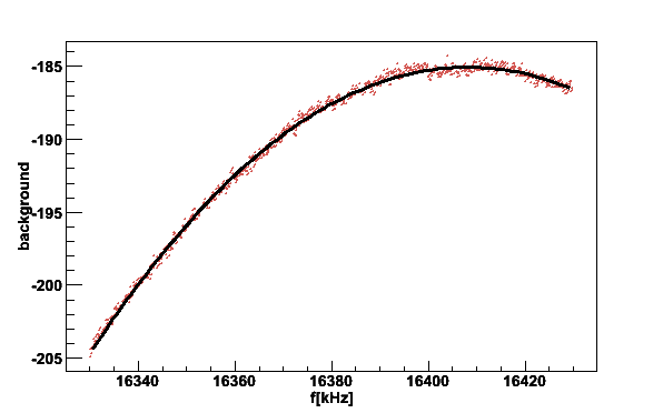
Fig 5. Baseline or the Q-curve. The black line is fit to a LCR function. The Q-value is about 22 and center frequency 16408 kHz.
Next we plot all the butanol coils from 2006 using pcoils, which
actually calls the plotsig to produce the plots. The given
parameters are passed to the plotsig.
pcoils -060614_190105.sig -b060614_174630.bgr -w300 -v2
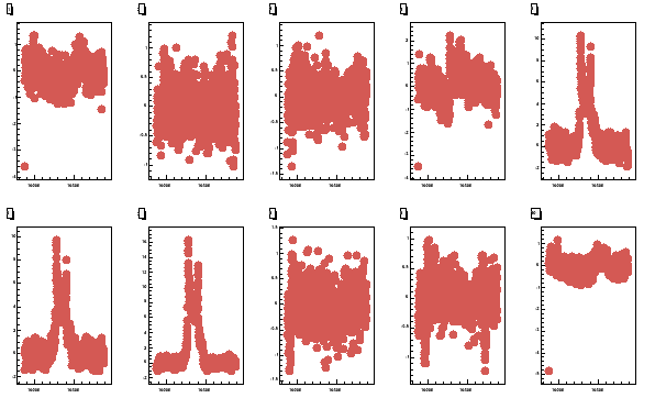
Fig 6. All the 10 butanol coils. The top row has coils 1 - 5 and bottom 6 - 10.
The peaks in the butanol signal can be found with option -M by
giving the threshold 0 - 1 as parameters. The peak search is based on the
Root TSpectrum
class. In the following example only the position of the first peak is printed
(this can be modified in the code)
plotsig -060614_190105.sig -b060614_174630.bgr -N5 -w300 -M0.7 -v2
        f0      A       M2      M4      a       chi
Raw     16350.7 936.538
Search 1 peaks sigma=1 threshold=0.7
f0      hist    sig
16280.7 10.0079 8.87846
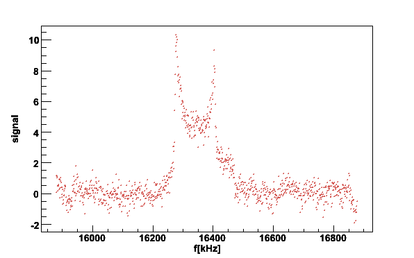
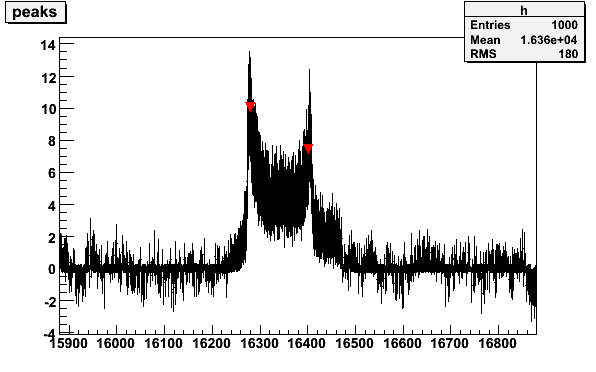
Fig 7. Butanol signal with histogram to determine the position of the peaks.
Multiple signals can be plotted into one plot with msig. First
the files to be plotted are given in a list file, for example
070420_145601_16swp.bgr
070420_160058.sig
070420_180117.sig
070420_200137.sig
The plot command could then be
msig -pTEfiles -Pprot/ -w200 -v2
here the TEfiles is list of the signal files to be plotted and prot is the path to find the files.
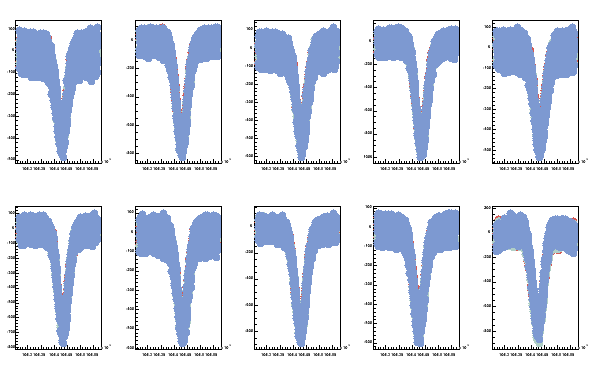
Fig 8. Three proton TE-signals superposed in one plot. All 10 coils are shown.
As an example we want to analyze the NMR signals during the 2006 polarization build up from September 13 to 14. First we need to create a list of the signal files
cd /home/NMRdata/2006/2006CD1
ls Sep13-14pol/* > Sep13to14files
Next we edit the file Sep13to14files to select the interesting
time region. First line in this file has to contain the
bgr file. Next we take the integral of the raw signal and
the first moment after removal of a linear baseline for each coil
excluding 40 kHz from the center in the baseline fitting. In addition
the unix time stamp is given for each analyzed file.
The results are written in file Sep13to14fA.
The switch -P gives the path to the files to be analyzed.
With the '&' at the end of the line the calculation moves
to background and you can leave it running.
loopsig -Sep13to14files -P/home/NMRdata/2006/2006CD1/ -s40 -u > Sep13to14fA &
We check the progress of the calculation with tail command
tail -f Sep13to14fA
You can check the process number for loopsig with
ps command and stop the process any time with
kill using the process number.
After the calculation has finished we plot
the integrated area for all the coils
plotpar -Sep13to14fA -ifA -pA -t10000
The switch -ifA tells that the file contains the
first moment frequency and the integrated area for each coil.
-pA tells to plot the area and -t10000
gives the y-position for the coil marker legend.
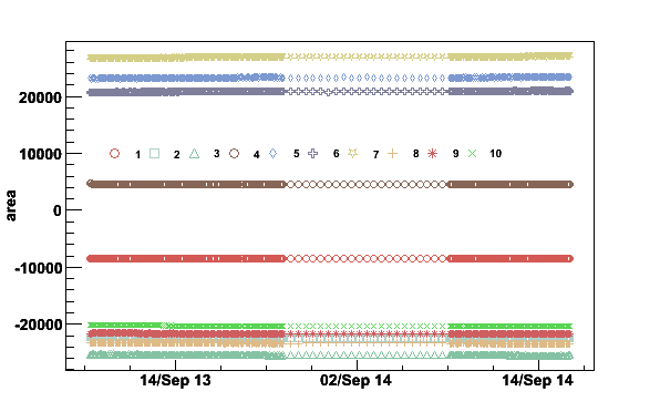
Fig 9. Integrated areas September 13 to 14 2006.
Next we plot the first moments for all the coils to see if the magnetic field was stable during the polarization buildup
plotpar -Sep13to14fA -ifA -pf -t16341
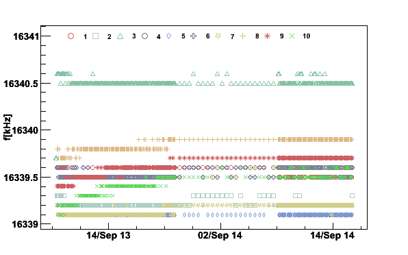
Fig 10. NMR signal first moments September 13 to 14 2006.
The data can be plotted also in histogram with histpar.
histpar -Sep13to14fA -ifA -pf -b10 > Sep13to14ffmap
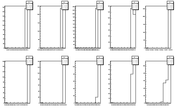
Fig 11. Histogram of first moments September 13 to 14 2006. The coils on the top row are 1 to 5 and on the bottom 6 to 10.
The median, 18.5 % and 81.5 % quantiles are now saved in the file
Sep13to14ffmap. This can be plotted for the coil positions
of the three target cells 2006. We plot the NMR center frequency as a
magnetic field by giving the isotope parameter -BD in
mappar -Sep13to14ffmap -pf -e -3 -BD -t2.5001
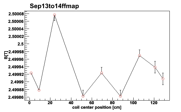
Fig 12. NMR signal first moments for different coils September 13 to 14 2006. The asymmetric error bars are given by the 18.5 % and 81.5 % quantiles. Coil #4 is neglected for 2006.
The thermal equilibrium NMR signals are analyzed by integrating the surface area of the signal after the linear baseline has been subtracted. First we create a list of the NMR files for one temperature with
ls TE1_0KJul/* > te1kfilesJul06
Next step is to edit the listfile to select the period for good thermal
equilibrium. The first file must be background file. Then we analyze these
files with loopsig. The options below give only the
integrated areas -I, linear baseline is fitted by excluding
40 kHz from the center and unix time stamp is given:
loopsig -te1kfilesJul06 -s40 -u -I > te1kareas40sJul06 &
First you can plot the signals one by one on the screen with option
-G to check that they look good and only after that
put the process to background. In this case you can press Alt-F and
then Q from the keyboard to close the graphics window.
The same procedure is repeated to all the temperatures. Then a TE-file
is created for the tecalc program. Here is an example
of the 2006 TE-file:
1.1238 0.004
te1kareas40s100lJul06
1.4139 0.0026
te1k4areas40s100lJul06
1.5985 0.0029
te1k5areas40s100lJul06
1.5068 0.00235
te1k5areas40s100lSep06
1.0182 0.0051
te1k0areas40s100lSep06
First line has spin temperature for that period and the error in the spin temperature, both in Kelvins. The analysis of all the TE-calibration data is done with
tecalc -TE06file -p
Histogram median
-1622.43 -4558.94 -5195.12 -2394.25 -4714.28 -4328.31 -5278.62 -4494.81 -4352.97 -3479.1
The printed values are the medians from the area times temperature histograms.
With the option -p also the histograms are plotted
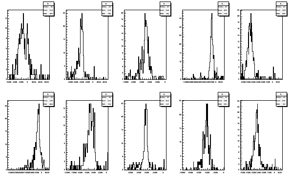
Fig 13. Area times temperature histograms from 2006 TE-calibration for all the coils.
To determine the polarization the surface areas for the NMR-signals need to
be integrated. This is done also with loopsig. For example
we want to know the polarization from August 23 to 24 in 2006.
First we create list file from the enhanced signals
ls Aug23-24pol/* > Aug23to24files
Next the list file is edited. The first file in it must be a background file. Then the areas are calculated
loopsig -Aug23to24files -P/home/NMRdata/2006/2006CD1/ -s40 -u -I > Aug23to24areas &
For polarization calculation we need to know also the Curie constants
from the thermal equilibrium calibration and the DC gains used during this
calibration. These are kept in files curie_file and
gain_file. For example files could be
-1792.38
-4497.78
-5255
-2178.82
-4905
-4240
-5372.73
-4551.58
-4410.32
-3627.83
and
212.829
212.671
211.711
210.889
206.42
204.932
210.698
211.374
211.257
213.443
Finally we calculate the average cell polarizations for the three target cells. The center frequency 16340 kHz needs to be given to calculate the thermal equilibrium polarization at 1.0 K temperature.
a2pol -Aug23to24areas -tcurie19Oct06jaakko -ggain19Oct06kaori -f16340 -3 -S
1156317617 -53.5131 51.1092 -57.2184
1156317919 -53.5775 51.2015 -57.2089
1156318120 -53.4679 51.0971 -57.2179
1156318724 -53.6196 51.2623 -57.2572
1156319329 -53.6633 51.2734 -57.2794
...
As an example we want to plot the polarization from Kaoris offline file.
First it needs to be translated to unix format and we take only
average polarization of each of the three target cells with option
-3.
polk2j -j06allJan -u -3 -S > newpolfile
If there are problems in this conversion you should use verbose
level 1 or more to see where the problems come from. This is done
with the switch -v. The different SPS periods are
given in file run2006pers, for example for 2006
2006

PERIOD
P1B 7 21 8 8 14 0
P1C 8 14 8 8 30 0
P2A 8 30 8 9 19 0
P2B 9 19 8 10 2 0
P2C 10 2 0 10 18 16
P3A 10 18 16 11 8 8
P3B 11 8 8 11 20 0

MD
7 26 8 7 26 16
8 2 8 8 4 16
8 23 8 8 25 8
8 30 8 8 31 8
9 4 8 9 6 8
9 13 8 9 14 16
9 19 8 9 20 16
9 26 8 9 27 8
10 4 8 10 5 8
10 11 8 10 11 16
10 17 8 10 18 16
10 24 8 10 25 16
10 31 8 11 2 0
11 7 8 11 10 0
11 14 8 11 17 0

TR

TE
7 11 16 7 16 8
9 21 16 9 26 0
11 23 8 11 24 9
Here the period start and end months, days and hours are given. Since there was
no transversity data taking no start and end times are given after
TR.
With these the one year polarization plot is then produced
plotper -newpolfile -prun2006pers -S -3 -t1.3The switch
-S tells to include the solenoid current to the plot,
-3 average polarization for each target cell and
-t1.3 gives the position of the title from the top of the plot.
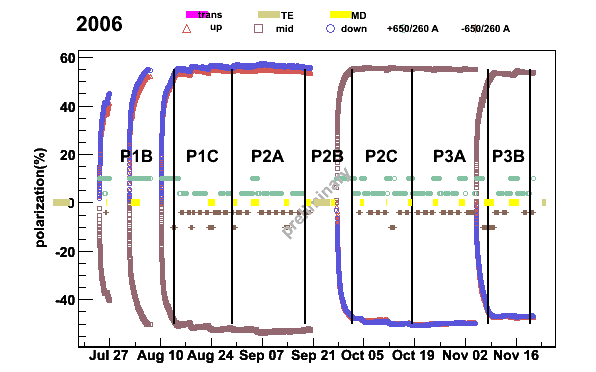
Fig 14. 2006 polarization from SPS periods P1B to P3B.
The runpol can be used to interpolate the polarization values
for each run in the run logbook database. It needs the run number file with
run start and stop time in addition to run type. This file can be created with
mysql client, for example
QUERY="select runnb,starttime,stoptime,runtypeid from tb_run where starttime >= '2007-05-01' and starttime <= '2007-10-01' ;"

echo $QUERY | mysql -u user -h host_name runlb > RunNbs
With the SPS period file run2007pers the frozen spin polarization
values can be interpolated
runpol -pol07.apol -rRunNbs -prun2007pers > pol07.run
The run numbers with week name can be obtained with
"select runnb,period from tb_chunklist where runnb>=63000 and runnb <= 64001;".
The duplicate run numbers need to be removed from this file and the result
sorted with the run number. The result is written to a file
RunPers. Finally the week 36 from 2007 can be plotted
plotweek -pol07.run -wRunPers -S -P -T -t1.15 -a0.8 -W36
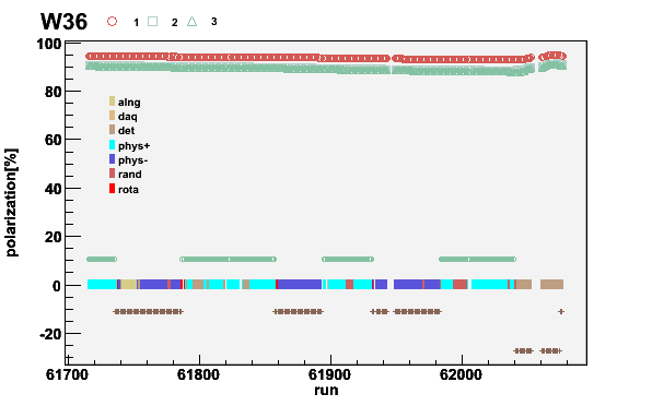
Fig 15. Week 07W36 polarization. The negative polarizations are plotted as positive for clarity. The missing runs or runs without end time are empty. The solenoid current is shown with the brown/green points around zero.
Here is a xy-plot between integrated signal area and center frequency using
plotpars. The switch -i gives the list of the
parameters in the file, -x parameter on x-axis and
-y parameter on y-axis.
plotpars -Df0areas -ifA -xA -yf
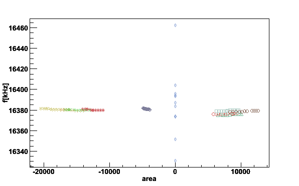
Fig 16. The first moment center frequency vs. integrated area.
Next we want to plot temperature of TTH4, TTH5 and TTH6 into one plot.
For this we merge the the files first with parmerge and finally
plot the results with plotpar
parmerge -TE07Nov1K3.tth4 -DTE07Nov1K3.tth5 > TE07Nov1K3.tth45

parmerge -TE07Nov1K3.tth45 -DTE07Nov1K3.tth6 > TE07Nov1K3.tth456

plotpar -TE07Nov1K3.tth456 -iRT -pT -L -g
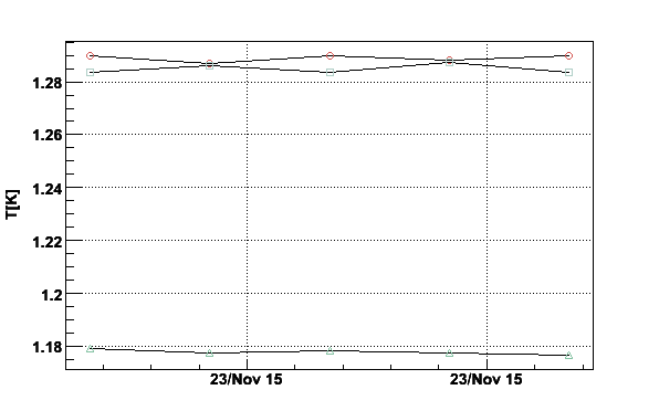
Fig 17. Plot of temperature given by TTH4, TTH5 and TTH6.
The parmerge can also be used to select a wanted time period
from the file.
The plotpar can be used to find minimum rms noise line from the
TE-area plot, where the spin system is most likely in thermal equilibrium with
the helium. For this the switch -c is used. It defines the
number of cuts to try in the windows [0,start] and [end,1], where
0 <= start < end <= 1. Robust quantile method is used to estimate the minimum
rms value. The best fit is taken from a period of lowest average rms noise for
all the coils.
plotpar -TE3-1K3_071115.raw -ifA -pA -t-20000 -c0.18,10,0.3,0.9,10 -v1 -Ttesting
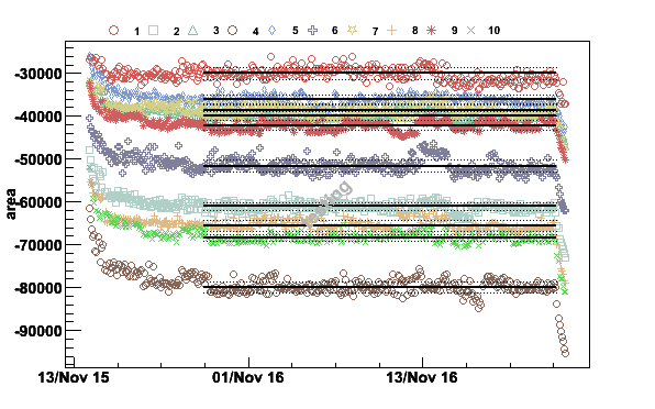
Fig 18. The spin system has reached thermal equilibrium around 22:00 on November 15.
For simulation of the NMR signal first signal description file needs to be written. Here is an example for proton TE-signal
PNTS 1000
FSTART 106118
FSTEP 0.6
QAMP -3.57256e+08
Q 6.1754
QF0 106416
QOFF 9.37753e+06
QNOISE 20
TYPE NH3
M2  441.931
F0 106437
AMP -724.935
1000 points are generated starting from 106118 kHz using steps of 0.6 kHz.
The Q-curve is defined with parameters QAMP, Q,
QF0, QOFF and QNOISE. The NMR signal
type is NH3 with second moment M2, center frequency
F0 and amplitude AMP.
The simulation is then done with simsig. The result is piped to
plotsig, which is also used to fit the signal to a gaussian.
The TRandom3
class is used to generate the random numbers.
simsig -simnh3pars | plotsig -stdin -bstdin -w300  -v2 -N1 -fG -L1
...
        f0      A       M2      M4      a       chi
Raw     106434  -68384.2
Gaus    106437  -65872.8        466.29 -                -730.196        865708
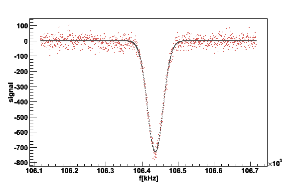
Fig 19. Plot of the simulated proton signal with gaussian fit.
To simulate complete thermal equilibrium calibration with the same number of background and signal files as in the real TE-calibration an additional file is needed
1.5136 0.0014
list1K5
1.0169 0.0015
list1K0
Here the temperature and temperature error are given. This is followed by
a list file of the background and signal files. The simulated signals are
piped directly to tecalc to see the results
simte -simnh3pars -tTEprot -o | tecalc -stdin -N1 -b10 -q0.18 -p -e
-63232.2
1.86584
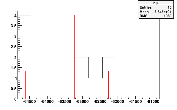
Fig 20. Histogram from simulated TE-calibration with 13 signal files and 6 background files.
Many TE-calibrations can be simulated with msimte, for example
10 calibration with the same NMR- and TE-simulation files as above using
histpar to plot the results in a histogram.
msimte -simnh3pars -tTEprot -N10 > mCuries
histpar -mCuries -iA -pA -1 -b10
-64116.9
-65414.6
-61619.5
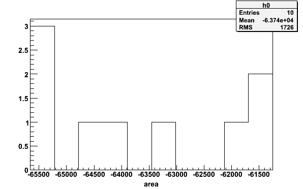
Fig 21. Histogram of 10 simulated Curie constants.
The flow diagram of the thermal equilibrium analysis simulation is show below.
The msimte calls simte as many times as given
by the switch -N. The simte reads first the
TE-file for the temperatures and temperature errors. The names of the
list files are also given. The number of backgrounds and signals are counted
from the list files. The simte calls then simsig
and uses switch -a to scale the signal according to the
temperature. The simsig reads the NMR-signal and Q-meter
parameters from a file and sends the simulated background followed by
signal to the plotsig. The plotsig integrates the
area and first moment and returns the values back to simte.
The simte sends the integrated area values
to tecalc and reads back
the analyzed Curie constants. The msimte gets the values and
writes the simulated Curie constants
to standard output with a unix time stamp.
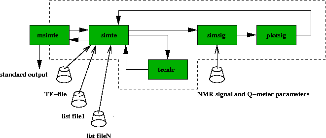
Fig 22. Flow diagram for simulation of the TE-analysis. The user is
interacting only with msimte, which then calls the other programs.
Different dilution cryostat parameters can be extracted with the
mulreg utility. For example the 3He vapor pressure
temperature from the baratron pressure gauge
mulreg -test3HeP -tBARATRO -p -T
15/01/08 15:16:30 5.325453e-2    71.00   0.6005
15/01/08 15:16:30 1.350115e-1   180.00   0.7001
15/01/08 15:16:30 2.835241e-1   378.00   0.8001
15/01/08 15:16:30 5.212943e-1   695.00   0.9001
15/01/08 15:16:30 8.700740e-1  1160.00   1.0000
15/01/08 15:16:30 1.353212  1804.13   1.1000
15/01/08 15:16:30 1.990669  2654.00   1.2000
15/01/08 15:16:30 2.803738  3738.00   1.3000
15/01/08 15:16:30 3.811074  5081.00   1.4000
15/01/08 15:16:30 5.032178  6709.00   1.5000
15/01/08 15:16:30 6.487301  8649.00   1.6000
After the time stamp there is the voltage read from the baratron, pressure in Pascals and corresponding temperature in Kelvins. In this example all the points had the same time stamp, which is usually not the case.
The levpops can be used to check the polarization of other
isotopes in the target material. For example for deuteron target assuming
equal spin temperature
levpops -iD -p50 -B2.5 -m -v1
f0=16340 kHz
Spin 1 Ts=0.00094016 K

E+ -------- p+ 11.621 %
E0 -------- p0 26.76 %
E- -------- p- 61.621 %

p  99.1303 %
6Li 48.3137 %
7Li 90.8765 %
The polrlx can be used to calculate the polarization relaxation in
frozen spin target. For example deuteron target of 40 mols polarized to 50 %,
heat flow of 2 nW to the spin system in 2.5 T after 7 days gives
polrlx -iD -p50 -Q2 -B2.5 -n40 -d7 -v1

Polarization 49.535 % after 7 days, relaxation 0.0664298 %/day
The momLiD can be used to calculate the second moment of the
NMR line of a given number of crystals and samples. For example for deuteron
with 10 crystals of random orientation and 10 samples
momLiD -iD -L11 -C10 -N10 -v1
2nd moment 2.27246 +- 0.265058 kHz^2
First increase the verbose level with switch -v to see where the
problem is coming from.
If the Root libraries are not found, you need to set the
LD_LIBRARY_PATH environmental variable, for example
> export LD_LIBRARY_PATH /afs/cern.ch/sw/lcg/external/root/5.12.00e/slc3_ia32_gcc323/root/lib
See the Root documentation how to do this.
[1] K. Kondo et al., Polarization measurement in the COMPASS polarized target, Nucl. Instr. Meth. A526 (2004) 70.
[2] J. Koivuniemi et al., NMR line shapes in highly polarized large 6LiD target at 2.5 T, Nucl. Instr. Meth. A526 (2004) 100.